
filmic rgb
Technical information
- description
- apply a view transform to prepare the scene-referred pipeline for display on SDR screens and paper prints while preventing clipping in non-destructive ways.
- purpose
- corrective and creative.
- input
- linear or non-linear, RGB, scene-referred.
- processing
- non-linear, RGB.
- output
- non-linear, RGB, display-referred.
Remap the tonal range of an image by reproducing the tone and color response of classic film.
This module can be used either to expand or to contract the dynamic range of the scene to fit the dynamic range of the display. It protects colors and contrast in the mid-tones, recovers the shadows, and compresses bright highlights and dark shadows. Highlights will need extra care when details need to be preserved (e.g. clouds).
darktable offers three modules for this task: filmic rgb, sigmoid and AgX. Only one of them should be enabled at a time. filmic rgb gives you the most direct control over where the black and white points of the scene are placed, at the cost of a larger number of parameters. The module is derived from another module of the same name in the Blender 3D modeller by T. J. Sobotka.
You can automatically enable this module in new images by setting the value of preferences > processing > auto-apply pixel workflow defaults to ‘scene-referred (filmic)’.
Note: The controls of this module look technical, but they are meant to be set by eye. Judge the result on the image, not on the numbers in the GUI.
🔗before you start
filmic rgb expects a linear, scene-referred image with a sensible mid-tone level. Prepare the image as follows:
- set the mid-tones
- In the exposure module, raise or lower the exposure until the mid-tones look right. Ignore the highlights at this stage – filmic rgb will bring them back.
-
Avoid negative pixel values in dark areas, as they make the calculations in filmic rgb unpredictable. On some camera models (mainly Canon), rawspeed – the raw decoding library of darktable – sets an exaggerated black level, which crushes the blacks and produces negative values. In that case, enter a negative black level correction in the exposure module.
- use only one tone mapper
- filmic rgb is a tone mapper; you typically have exactly one tone mapper enabled for an image.
- prepare the image if you use the pickers
- The pickers in the scene tab measure luminance in RGB, where luminance and chrominance are linked. For reliable readings, first neutralize any color cast in the color calibration or white balance module, use a high quality demosaic algorithm and denoise a noisy image beforehand. None of this is required if you set the exposure sliders by hand.
Note: The module works best on images that use the full dynamic range of the sensor. In-camera, expose as brightly as the highlights allow (a technique known as “expose to the right”). Some clipping is acceptable – for example on specular reflections – but clipped data is lost and can only be approximated, using the reconstruct tab.
🔗how filmic rgb works
filmic rgb maps the dynamic range of the photographed scene to the dynamic range of the display. The mapping is defined in five tabs:
- The scene tab defines the input: which luminances in the scene are to be treated as white and as black.
- The reconstruct tab handles blown highlights.
- The look tab defines the artistic intent. It applies an S-shaped curve that increases mid-tone contrast and maps the scene’s middle-gray to the middle-gray of the display.
- The display tab defines the output. These parameters rarely need to be changed.
- The options tab contains advanced settings. filmic rgb compresses local contrast. Once you are happy with the tone mapping, you may want to compensate for this in the local contrast module, add saturation in the color balance rgb module, and refine the tonal distribution with the tone equalizer.
The sliders are limited to typical and safe values. To enter a value outside these limits, right-click the slider and type it in.
Note: filmic rgb always changes the image to some degree – there is no neutral setting. The following comes close, and performs little more than a logarithmic mapping between the bounds set in the scene tab:
- in the look tab, set contrast to 1.0, linear region to 99% and highlights saturation mix to 0%,
- in the options tab, set contrast in shadows and contrast in highlights to soft.
🔗graphic display
The graph at the top of the module offers several views. Cycle through them with the
 icon to the right of the graph, and toggle the axis labels with the
 icon.
icon.
- look only
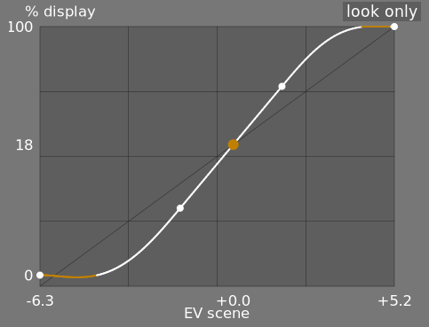
- This is the default view. The main bright curve shows how the dynamic range of the scene (in EV) is compressed into the display-referred output range. The orange dot shows the middle-gray point and the white dots either side mark out the linear region.
-
- look + mapping (linear)
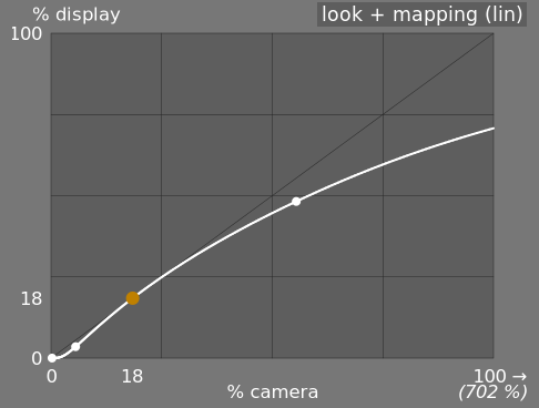
- This view shows the mapping of input values [0,1] to output values in linear space, including the dynamic range mapping and the output transfer function. In a scene-referred workflow input values may exceed 1, but the graph is limited to the interval [0,1]. The actual value of the scene white point is shown in brackets on the X axis, expressed as a percentage of an input value of 1.
-
- look + mapping (log)
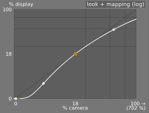
- The same as the previous view, but plotted in log space.
-
- dynamic range mapping
- This view is inspired by the Ansel Adams Zone System, showing how the zones in the input scene (EV) are mapped to the output. Middle gray from the scene is always mapped to 18% in the output (linear) space, and the view shows how the tonal ranges towards the extremes of the scene exposure range are compressed into a smaller number of zones in the display space, leaving more room for the mid-tones to be spread out over the remaining zones. The linear region is represented by the darker gray portion in the middle.
-

The look views also warn you when the curve is not usable:
- An orange section at the bottom or top of the curve means that the spline overshoots the limits of the display.
- A red dot means that the linear region is pushed too far towards the top or the bottom.
- A dot drawn as a half circle means that contrast is too low for the dynamic range of the image. In each case filmic rgb sanitizes the parameters internally, but the result is no longer what the sliders suggest. See troubleshooting for the corrective actions.
🔗module controls
🔗scene
The scene tab defines black, gray and white for the photographed scene. It is comparable to a levels tool, except that it works on scene-referred values in EV rather than on display-referred percentages.
- white relative exposure
- The number of stops (EV) between the scene middle-gray luminance and the scene luminance to be remapped to display white (peak-white). This is the right bound of the scene dynamic range that will be represented on the display – everything brighter than this value on the scene will be clipped (pure white) on the display. The picker tool reads the maximum luminance in RGB space over the drawn area, assumes it is pure white, and sets the white exposure parameter to remap the maximum to 100% luminance.
- black relative exposure
- The number of stops (EV) between the scene middle-gray luminance and the scene luminance to be remapped to display black (maximum density). This is the left bound of the scene dynamic range that will be represented on the display – everything darker than this value on the scene will be clipped (pure black) on the display. This slider therefore controls how far the shadows are recovered.
-
The picker tool reads the minimum luminance in RGB space over the drawn area, assumes it is pure black, and sets the black exposure parameter to remap the minimum to 0% luminance. This measurement is very sensitive to noise and cannot tell actual black apart from noise. It works best on low ISO images with high quality demosaicing. A resulting value of –16 EV means that the measurement has failed and the value has to be set by hand.
- dynamic range scaling and auto-tune
- The auto-tune picker combines the above pickers, and allows you to set the white and black exposures at the same time, using the maximum of the drawn region as the white and the minimum as the black. This gives good results in landscape photography but usually fails for portraits and indoor scenes.
-
When no true white and black are available on the scene, the maximum and minimum RGB values read on the image are not valid assumptions any more. Dynamic range scaling symmetrically shrinks or enlarges the detected dynamic range and the current parameters. This works with both pickers, and adjusts the current values of white and black relative exposures.
- middle-gray luminance (hidden by default)
- This slider defines which luminance in the scene is treated as middle-gray and remapped to 18% on the display. Use the exposure module for this instead – that is why the slider is hidden. To show it, enable use custom middle-gray values in the options tab.
-
Changing this value acts like a brightness correction. High values preserve the highlights but recover little shadow detail; low values recover the shadows but compress the highlights more harshly and reduce local contrast. The white and black relative exposures are adjusted automatically to keep the dynamic range from clipping, and can be corrected afterwards.
Note: The dynamic range shown here (white EV minus black EV) is not the dynamic range of your sensor as measured by DxOMark or PhotonsToPhotos. Several modules process the image before filmic rgb, so its input has a theoretically infinite dynamic range. The value only describes pixel encoding, not sensor capability.
The scene-referred workflow applies a black level correction of –0.0002 in the exposure module, which usually results in a dynamic range of around 12.3 EV at the input of filmic rgb. If a black relative exposure of –16 EV still fails to unclip the blacks, lower that correction further.
🔗reconstruct
The controls in this tab blend the transition between clipped and unclipped areas and can reconstruct color from adjacent pixels. They are designed for small light sources that could not be exposed differently – a bare light bulb or the sun in the frame – and diffuse their edges in the way film would. They are not designed to recover large clipped areas or to in-paint missing parts of the image.
Disabling the highlight reconstruction module gives the algorithm more data to work with, since that module clips highlight data by default. This may produce magenta highlights, which can be corrected with the gray ↔ colorful details slider.
Reconstruction works in two steps: first define a mask that identifies the areas to be treated, then balance the trade-offs of the reconstruction algorithm.
🔗highlights clipping
These controls define which areas of the image the reconstruction algorithms are applied to.
- enable highlight reconstruction
- Highlight reconstruction is disabled by default, for performance reasons, and should only be enabled when required. It is also enabled automatically as soon as the threshold or transition sliders are adjusted.
- threshold
- Pixels brighter than this threshold are treated by the reconstruction algorithm. The unit is EV, relative to the white point set in the scene tab. Enable display highlight reconstruction mask and adjust the threshold until the areas you want to reconstruct are shown in white. The raw overexposed warning shows you beforehand which pixels are clipped in the raw file, and whether they are clipped in one channel or in all of them.
- transition
- This control softens the transition between clipped and valid pixels. Moving it to the right blurs the mask, producing a smoother blend; moving it to the left sharpens the mask and reduces the feathering.
- display highlight reconstruction mask
- Click the icon to the right of this label to show the reconstruction mask. Keep it enabled while adjusting the two controls above.
🔗balance
These controls balance the trade-offs between the reconstruction algorithms.
- structure ↔ texture
- This control decides whether the algorithm paints in a smooth color gradient (structure) or reconstructs texture from sharp detail found in unclipped pixels (texture). The default of 0% favors both equally. Where all three channels are clipped, no texture is available – move the slider to the left. Where only one or two channels are clipped, the remaining channels still carry detail – move the slider to the right.
- bloom ↔ reconstruct
- This control decides whether the algorithm reconstructs sharp detail in the clipped areas (reconstruct) or applies a blur that approximates the blooming of traditional film (bloom). The default of 100% maximizes sharpness. Moving the slider to the left adds blur, which tends to darken the highlights and may make the reconstruction more colorful.
- gray ↔ colorful details
- This control decides whether the algorithm recovers monochromatic highlights (gray) or colorful ones. Move it to the right for more color in the highlights, to the left to desaturate them. Desaturating helps when magenta or out-of-gamut colors appear.
🔗look
The look tab shapes the S-curve. Watch the look only graph while adjusting it: the curve should rise smoothly from the black point at the bottom left to the white point at the top right. If it does not, see troubleshooting.
- contrast
- This slider controls the slope of the middle, linear part of the curve, and therefore mostly affects the mid-tones. The larger the dynamic range of the scene, the more contrast is needed for a natural-looking image. Note that global contrast also affects acutance – a low-contrast image looks unsharp even when it is optically sharp in the sense of the Optical Transfer Function (OTF).
-
A value of 1 almost completely disables the S-curve, leaving only a small residual effect from the splines in the shadows and highlights.
-
The curve is built by computing virtual nodes from the module parameters and interpolating between them. It consists of a linear middle part and two ends that transition smoothly to the limits of the exposure range. Unlike in a curve module, the nodes cannot be moved manually.
- linear region
- The range around middle-gray that is mapped with the slope set by contrast, expressed as a percentage of the dynamic range defined in the scene tab. This is the luminance range that is rendered with priority – and also the range that is not desaturated at the extremes (see highlights saturation mix).
-
As a rule of thumb, make the linear region as large as the curve allows. Whatever is not covered by it has to be handled by the two compressed ends of the curve, so a larger linear region means more of the image is rendered at the contrast slope.
-
There is a limit, though: enlarging the linear region leaves less room for the ends of the curve, which then start to overshoot. Enlarge it until the graph warns you, then back off. If you need more room at one end only, shift the region with shadows ↔ highlights balance instead of shrinking it; reducing the contrast also relaxes the constraint.
- shadows ↔ highlights balance
- By default the linear region is centered on the dynamic range. This slider shifts it towards the shadows or the highlights, giving one end of the tonal range more room than the other.
- highlights saturation mix
- At the extremes of the tonal range, pixels tend towards pure white or pure black, neither of which can carry saturation. This slider controls how that transition is made. Positive values keep the highlights saturated – suitable for skies, but to be used with care on skin tones. Negative values bleach the highlights. The default of 0 mixes both strategies.
-
Since the gamut mapping introduced in v6 handles the extremes accurately, there is no longer a separate desaturation curve to shape. In practice this slider is now a bleaching control for the highlights.
-
It is not intended for creative saturation. Handle saturation earlier in the pipeline instead, for example with the “add basic colorfulness” preset in the color balance rgb module. The technical background is described under gamut mapping.
- hardness (hidden by default)
- The power function applied to the output transfer function. It is calculated automatically from the values in the scene tab. To set it by hand, disable auto adjust hardness in the options tab.
-
This parameter is often called “gamma”, a term that is ambiguous in imaging and is avoided here. It raises or compresses the mid-tones to account for display non-linearities and to avoid quantization artifacts in 8-bit output. Output ICC profiles normally perform this step themselves, but the signal leaving filmic rgb is logarithmically encoded, which those profiles do not account for. filmic rgb therefore pre-compensates so that middle-gray is mapped to 45% instead of 76%.
🔗display
The parameters in this tab rarely need to be changed. They define the target luminances of the output medium. Note that darktable uses the same pipeline for the display preview and for the exported file.
- target black luminance
- The black level of the target medium. The default is the lowest non-zero value that the output color space can encode. Setting it to zero maps some non-zero luminances to 0 and may lose detail in the deepest shadows. Raising it produces faded blacks for a “retro” look. Non-zero values also constrain the S-curve and can make it harder for filmic rgb to find a smooth spline.
- target white luminance
- The white level of the target medium. Values below 100% produce muted whites for a “retro” look.
- target middle-gray (hidden by default)
- The middle-gray of the output medium, used as the target for the central node of the S-curve. On gamma-corrected media the effective value is computed as middle-gray^(1/gamma), so 18% with a gamma of 2.2 results in an actual target of 45.87%. This duplicates the exposure control in the exposure module, which should be used instead.
Note: The default values are correct for almost all purposes. The exception is output in a linear RGB space (Rec. 709, Rec. 2020) intended for media that handle log-encoded data. To remove the compression described under hardness, set the hardness to 1.0 and the target middle-gray to 45%.
🔗options
- color science
- Defines the algorithms used by filmic rgb. New edits use v7 (2023), which is the version described on this page. Images edited with an earlier version keep that version so that existing edits are not changed. See legacy color science for the older variants.
- contrast in highlights
- The curvature at the highlights end of the spline. safe never over- or undershoots but has muted contrast near white. The default, hard, constrains the slope more tightly, giving a sharper curve and more tonal compression in the highlights. soft relaxes the constraint for a gentler curve with less compression.
- contrast in shadows
- The same for the shadows end of the spline. safe never over- or undershoots but has muted contrast near black, hard (the default) compresses the shadows more, and soft compresses them less.
-
Which setting to choose: Keep hard unless the graph shows a problem – it suits most scenes. Switch the affected end to soft if that end looks over-compressed, or if you want to enlarge the linear region further. Switch it to safe if the spline keeps overshooting and the other adjustments have not helped: safe always produces a usable curve, at the price of muted contrast near black or white. The two ends are set independently, so change only the one that causes the problem.
- use custom middle-gray values
- Shows the middle-gray luminance slider in the scene tab. Disabled by default, since middle-gray should be set in the exposure module.
- auto-adjust hardness
- Enabled by default. When disabled, the hardness slider appears in the look tab.
- iterations of high-quality reconstruction
- The number of passes of the highlight reconstruction algorithm. The default reconstruction works on separate RGB channels in a single pass. The high-quality reconstruction works on RGB ratios and propagates color from neighboring pixels into the clipped areas over several passes, which produces more neutral highlights at a higher processing cost. It is useful where channel clipping has produced magenta highlights.
-
Too many iterations make the reconstruction degenerate: colors from further away bleed into the clipped areas – white clouds filled with blue sky, or the sun disc behind trees filled with leaf green.
- add noise in highlights
- Adds noise to the reconstructed highlights so that they do not look unnaturally smooth next to areas that still contain sensor noise.
- type of noise
- The statistical distribution of the added noise. poissonian noise is closest to natural sensor noise, gaussian is less faithful but visually more pleasing and closer to film grain. Most denoising modules turn sensor noise from poissonian to slightly gaussian, so choose whichever blends better into the noise actually present in the image.
🔗troubleshooting
🔗the curve is not smooth
If the graph shows an orange section, a red dot or a half-circle dot (see graphic display), the requested curve cannot be realized. Try the following, in this order:
- check that white relative exposure and black relative exposure in the scene tab actually match the scene,
- reduce the linear region and/or the contrast in the look tab, or increase the contrast if a dot is drawn as a half circle,
- shift the linear region with shadows ↔ highlights balance,
- set contrast in shadows and/or contrast in highlights in the options tab to safe or hard,
- reduce target black luminance in the display tab if it is not zero.
🔗the highlights have no color
Work through the causes in this order, because each one makes the next impossible to judge:
- Check the white relative exposure in the scene tab. If it is set below the brightest tones of the scene, those tones are clipped to pure white before any saturation control can act on them. No later setting can bring their color back.
- Check whether the highlights are clipped in the raw file itself, using the raw overexposed warning. Clipped channels carry no color information; see reconstruct.
- Only then raise highlights saturation mix in the look tab. High values can produce fringes around bright areas.
- If the highlights are neither clipped nor bleached but the image as a whole looks flat, add saturation in the color balance rgb module rather than here.
🔗color artifacts
filmic rgb preserves hue much more strictly than a simple per-channel curve. It is therefore less forgiving of invalid colors such as chromatic aberrations and clipped magenta highlights, which a per-channel curve would have hidden – though not solved.
A tone mapping operator cannot repair a damaged signal. Correct such defects earlier in the pipeline with the modules provided for the purpose. As a quick workaround, any color brighter than the white relative exposure degrades to pure white, so setting the white relative exposure slightly below the exposure of the clipped area will render it as clean white: if it is clipped at the input, let it be clipped at the output.
🔗different output for different color spaces
If you export the same image to sRGB and to Adobe RGB and compare both on a wide-gamut screen, the sRGB version has more desaturated highlights. This is expected. The sRGB gamut boundary lies closer to the neutral axis, so less chroma is available at a given luminance. It is a sign that the gamut mapping is working, not a bug.
🔗gamut mapping
Very bright and very dark colors cannot be highly saturated at the same time. The graph below shows the gamut of the sRGB color space at the constant hue of its green primary, with lightness on the vertical axis and chroma on the horizontal axis:

As lightness approaches pure black or pure white, the available chroma shrinks to zero. If colors are allowed to leave the gamut, they are clipped when converting to the display color space. That clipping preserves neither hue nor luminance, so highlights typically shift towards yellow and appear darker than their surroundings.
filmic rgb therefore performs a test conversion into the display color space. If the result falls outside the [0; 100]% range, it computes the maximum saturation available in gamut at that luminance and hue, and clips the color to that value. This keeps the hue constant throughout the whole tone mapping and gamut mapping operation while making full use of the available gamut. The hue used as a reference is the hue at the input of filmic rgb, before any tone mapping.
The gamut is taken from the output color profile, so the mapping adapts to any output space. Only matrix and matrix + curve(s) ICC profiles are supported. With LUT profiles the gamut mapping falls back to the pipeline working space (Rec. 2020 by default).
The remaining trade-off – how much saturation to keep in the highlights – is controlled by the highlights saturation mix slider in the look tab. It mixes between two strategies: preserving the ratios between the RGB channels relative to the max RGB norm, which keeps highlights saturated, and applying the curve per channel, which bleaches them. Whatever the setting, the output saturation is never allowed to exceed the input saturation.
🔗legacy color science
Images edited with an earlier version of filmic rgb keep the color science they were edited with, so that their rendering does not change. The color science setting in the options tab makes these versions available: v3 (2019), v4 (2020), v5 (2021) and v6 (2022). They differ in how they desaturate colors close to pure black and pure white:
-
v3 to v5 desaturate the extremes of the tonal range along fixed curves, which is a conservative approximation of the gamut boundary. The look only graph shows an additional, darker “desaturation curve” for these versions.
-
v6 introduced the measured gamut mapping described above.
-
v7 replaced the preserve chrominance setting with the single highlights saturation mix slider. In v3 to v6, the preserve chrominance setting selects the norm N by which the RGB channels are divided before the S-curve is applied to N, so that the ratios between the channels are preserved:
-
no applies the curve to each channel independently. This saturates the shadows and desaturates the highlights, which can help with out-of-gamut blues or reds.
-
max RGB uses the maximum of the R, G and B channels. This is the behavior of the original version of the module. It tends to darken blues, especially skies, and may produce halos or fringes where channels are clipped.
-
luminance Y uses a linear combination of the channels. It darkens reds and increases local contrast in them, and behaves poorly with saturated or out-of-gamut blues.
-
RGB power norm uses (R³ + G³ + B³)/(R² + G² + B²) and is usually a good compromise between max RGB and luminance Y.
-
RGB euclidean norm is independent of the working color profile and gives the same result in any RGB space. It desaturates the highlights more than the power norm and is probably closest to a color film look. Several controls have been renamed over time. The tooltips in darktable always describe the behavior of the version currently selected.
| current name | former name(s) |
|---|---|
| linear region | latitude |
| hardness | target power factor function |
| highlights saturation mix | extreme luminance saturation (v3, v6), mid-tones saturation (v4, v5) |