scopes
This module provides various graphical depictions of the developed image’s light levels or chromaticity.
Hover the mouse over the module to reveal buttons that can be used to adjust the display. The buttons on the left-hand-side are used to choose the display mode, from left-to-right: vectorscope, waveform, rgb parade and histogram. The buttons on the right-hand-side control how the plot for the current scope is drawn.
The height of the scopes module can be changed by clicking-and-dragging on the bottom edge or by holding down Shift+Alt while scrolling the mouse. The visibility of the module can be toggled with a keyboard shortcut (default Ctrl+Shift+H).
The scopes module is at the top of the right-hand panel by default but can be moved to the left-hand panel with preferences > miscellaneous > position of the scopes module.
For performance reasons, scopes are calculated from the image preview (the image displayed in the navigation module) rather than the higher quality image displayed in the center view. The preview is calculated at a lower resolution and may use shortcuts to bypass more time-consuming image processing steps. Hence the display may not accurately represent fine detail in the image, and may deviate in other ways from the final developed image.
🔗histogram
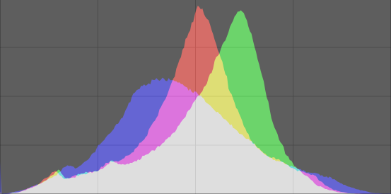
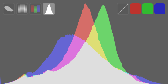
The histogram shows the distribution of pixels by lightness for each color channel.
The horizontal axis runs from 0% to 100% lightness for each channel. The vertical axis gives the count of pixels having the given lightness.
In its default state, data for all three RGB color channels is displayed. The red, green and blue colored buttons on the right-hand-side can be used to toggle the display of each color channel.
The first button on the right-hand-side toggles between logarithmic and linear rendering of the vertical axis (pixel count) data.
🔗waveform
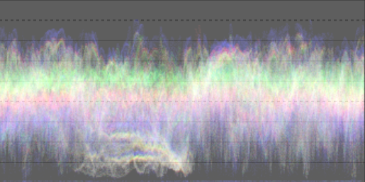
The waveform scope shows similar data to the histogram, but allows you to view that data in a spatial context.
In the “standard” horizontal waveform, the horizontal axis of the waveform represents the horizontal axis of the image – the right-hand side of the waveform represents the right-hand side of the image and the left-hand side of the waveform represents the left-hand side of the image.
The vertical axis represents the distribution of pixels by lightness for each channel – the dotted line at the top represents 100% lightness (values above this may be clipped), the dotted line in the middle represents 50% lightness, and the bottom of the waveform represents 0% lightness.
The brightness of each point on the waveform represents the number of pixels at the given position (the horizontal axis) having the given lightness (the vertical axis). The brighter the point, the more pixels at that position have that lightness.
As with the histogram, you can selectively display each of the red, green, and blue channels, by clicking on the appropriate buttons.
The first button on the right-hand-side toggles the display between horizontal (above) and vertical (below) mode:
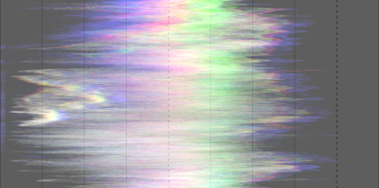
In the vertical waveform, the vertical axis of the plot represents the vertical axis of the image, and the horizontal axis represents the distribution of pixels by lightness. The vertical waveform can be useful for portrait-format images, or simply to understand an image in a different way.
See Of Histograms and Waveforms for more on darktable’s waveform scope.
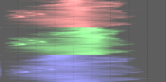
🔗rgb parade
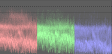
The RGB parade scope shows the same data as the waveform, but with the red, green, and blue channels presented side-by-side.
As with the waveform, clicking the button on the right-hand-side of the module toggles between horizontal (above) and vertical (below) mode:
The RGB parade can be useful for matching the intensities of the red, green, and blue channels. It can also help to understand the differences between, and individual qualities of, each channel.
🔗vectorscope
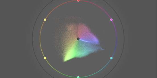
The vectorscope shows chromaticity without regard to either lightness or spatial data.
The distance from the center of the graph represents chroma and the angle represents hue. Areas of the graph are colored depending on the chromaticity of the color to which they correspond in the image. The graph represents color “volume” by rendering the more frequently used colors in lighter tones.
The graph includes a “hue ring” representing the maximum chroma of each hue (in bounded RGB) of the current histogram profile. The RGB primary/secondary colors are marked by circles around the edge of the hue ring.
🔗color harmony and additional vectorscope controls
The vectorscope provides some additional controls beyond those provided by the other modes, which deserve separate discussion. Hovering over the scopes module while in vectorscope mode shows the following additional buttons:
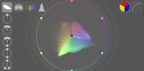
Click the right-most button to toggle the chroma scale between linear and logarithmic mode.
Click the second-to-right-most button to toggle the color space of the vectorscope between CIELUV, JzAzBz or RYB – as previously mentioned, these color spaces exclude any luminosity component in this module. The CIELUV graph will be faster to calculate, and is a well-known standard, though JzAzBz may be more perceptually accurate.
Finally, along the left-hand edge of the module are a series of buttons that allow the selected color harmony indicator to be overlaid on the vectorscope graphic when in RYB color space. For example, the following shows the “triad” color harmony:
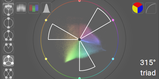
Rotate the display of the overlaid harmony guides by hovering over the scopes module and scrolling with the mouse scroll wheel. Hold Ctrl while scrolling to rotate more slowly. Hold Shift while scrolling to change the area covered by the guide overlays.
The type and position of the chosen harmony guides is saved alongside each image’s editing data (in the XMP file and database) so can be restored whenever you return to the image for further editing.
A full description of how to use this functionality is out of scope of this reference section, however, the following overview gives a basic guide as to how to use this mode to improve the color harmonies within the image.
-
With the global color picker, take live samples of the key colored areas of the image. The choice of these is purely artistic, depending on the feeling you wish to convey. Choose (in the global color picker) to display the chosen samples on the RYB vectorscope.
-
Choose the color harmony type that you wish to implement (or the closest to the actual distribution of picked live samples). Rotate (with Ctrl+scroll) until the picked samples fall roughly inside (or near) the harmony guides.
-
If some of the picked samples fall outside of the guide lines, perform manipulations of the image’s colors until they fall within the guides. You can use any processing module to achieve this but multiple masked instances of color balance rgb usually provide the best results.
Bear in mind that these controls are provided as a basic guide to achieving color harmony – do not try to force colors into the guides at the expense of the overall look of the image. For some useful examples of how to use this functionality, please see the pull request that implemented the original change.
🔗caveats
- The hue ring is not a gamut check, as a color can be within the hue ring, yet out of gamut due to its darkness/lightness.
- When adjusting an image based upon a color checker, faster and more accurate results will come from using calibrate with a color checker in the color calibration module.
- The vectorscope does not have a “skin tone line”, which is a flawed generalization rather than a universal standard.
- The vectorscope represents a colorimetric encoding of an image, which inevitably diverges from a viewer’s perception of the image.
🔗exposure adjustment
The histogram, waveform, and RGB parade scopes can be used to directly alter the exposure and black level of the exposure module.
For the histogram, click towards the right-hand side of the histogram and then drag right to increase or drag left to decrease the exposure. In a similar manner you can control the black level by clicking and dragging in the left-hand side.
For horizontal waveform and RGB parade, drag the upper portion of the scope up/down to increase/decrease exposure. Drag the lower portion up/down to increase/decrease the black level.
For vertical waveform and RGB parade scopes, the corresponding regions are to the right (exposure) and left (black level).
You can also scroll in the appropriate area – rather than dragging – to adjust exposure and black point.
Finally, you can override the default adjustment behavior as follows:
- hold Ctrl+Shift while adjusting to override the soft limits (e.g. to significantly overexpose the image)
- hold Ctrl while adjusting to fine-tune the adjustment. Alternatively, right-click to enter a precise value for the adjustment
- double-click on the desired area to reset to the original value
🔗histogram profile
Image data is converted to the histogram profile before the scope data is calculated. You can choose this profile by right-clicking on the soft-proof or gamut check icons in the bottom module and then selecting the profile of interest. When soft-proof or gamut check is enabled, the scope is shown in the soft proof profile.
As the scopes module runs at the end of the preview pixelpipe, it receives data in display color space. If you are using a display color space that is not “well behaved” (this is common for a device profile), then colors that are outside of the gamut of the display profile may be clipped or distorted.