curves
The base curve, tone curve and rgb curve modules use curves to control the tones in the image. These modules have some common features that warrant separate discussion.
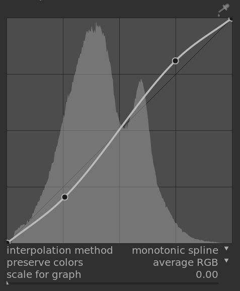
🔗nodes
In their default state, curves are straight lines, defined by two anchor nodes at the top-right and bottom-left of the graph. You can move the nodes to modify the curve or generate new nodes by clicking on the curve. Ctrl+click to generate a new node at the x-location of the mouse pointer and the corresponding y-location of the current curve – this adds a node without the risk of accidentally modifying the curve. Up to 20 nodes can be defined per curve. To remove a node, click on it and drag it out of the widget area.
🔗curve controls
The following controls are common to two or more of the above processing modules and are therefore discussed separately here. Please see the individual module documentation for discussion of any additional controls.
- interpolation method
- tone curve and rgb curve only
-
Interpolation is the process by which a continuous curve is derived from a few nodes. As this process is never perfect, several methods are offered that can alleviate some of the issues you may encounter.
-
- cubic spline is, arguably, the most visually pleasing. Since it gives smooth curves, the contrast in the image is better enhanced. However, this method is very sensitive to the nodes’ position, and can produce cusps and oscillations when the nodes are too close to each other, or when there are too many of them. This method works best when there are only 4 to 5 nodes, evenly spaced.
-
- centripetal spline is designed specifically to avoid cusps and oscillations but, as a drawback, it will follow the nodes more loosely. It is very robust, no matter the number of nodes and their spacing, but will produce a more faded and dull contrast.
-
- monotonic spline is designed specifically to give a monotonic interpolation, meaning that there will be none of the oscillations the cubic spline may produce. This method is most suitable when you are trying to build an analytical function from a node interpolation (for example: exponential, logarithm, power, etc.). Such functions are provided as presets. It is a good trade-off between the two aforementioned methods.
- preserve colors
- If a non-linear tone curve is applied to each of the RGB channels individually, then the amount of tone adjustment applied to each color channel may be different, and this can cause hue shifts. The preserve colors combobox provides different methods of calculating the “luminance level” of a pixel in order to minimise these shifts. The amount of tone adjustment is calculated based on this luminance value, and then this same adjustment is applied to all three of the RGB channels. Different luminance estimators can affect the contrast in different parts of the image, depending on the characteristics of that image. The user can therefore choose the estimator that provides the best results for the given image. Some of these methods are discussed in detail in the preserve chrominance control in the filmic rgb module. The following options are available:
-
- none
- luminance
- max RGB
- average RGB
- sum RGB
- norm RGB
- basic power
- scale for graph
- tone curve and base curve only
-
The scale allows you to distort the graph display so that certain graphical properties emerge to help you draw more useful curves. Note that the scaling option only affects the curve display, not the actual parameters stored by the module.
-
By default, a “linear” scale is used (defined by a scale factor of 0). This scale uses evenly spaced abscissa and ordinates axes.
-
A logarithmic scale will compress the high values and dilate the low values, on both the abscissa and the axis of ordinates, so that the nodes in lowlights get more space on the graph and can be controlled more clearly.
-
Increase the ‘scale for graph’ slider to set the base of the logarithm used to scale the axes. This allows you to control the amount of compression/dilation operated by the scale. If you draw purely exponential or logarithmic functions from identity lines, setting this value defines the base of such functions.