contrast equalizer
Adjust luminance and chroma contrast in the wavelet domain.
This versatile module can be used to achieve a variety of effects, including bloom, denoise, clarity, and local contrast enhancement.
It works in the wavelet domain and its parameters can be tuned independently for each wavelet detail scale. The module operates in CIE LCh color space and so is able to treat luminosity and chromaticity independently.
A number of presets are provided, which should help you to understand the capabilities of the module.
🔗module controls
The contrast equalizer module decomposes the image into various detail scales. On each detail scale, you can independently adjust the contrast and denoise splines for lightness (“luma”) and chromaticity (“chroma”, or color saturation), as well as adjusting the edge-awareness (“edges”) of the wavelet transform. The luma, chroma and edges splines are provided on separate tabs, and some examples of their usage are given in the following sections.
Below the spline graphs is a mix slider, which can be used to adjust the strength of the effect, and even to invert the graph (with negative values). While your mouse is over the spline graph, the curve will be displayed as if the mix slider was set to 1.0, to allow for easier editing. When you move your mouse away, the graph will be re-adjusted to account for the mix slider.
In the background of the curve you can see a number of alternating light and dark stripes. These represent the levels of detail that are visible at your current zoom scale – any details without these stripes are too small to be seen your current view. Adjustments made to control points within the striped section may produce a visible effect (depending on the strength of the adjustment). Adjustments outside of the striped region will not. Zoom in to see higher levels of detail and make adjustments to the more detailed areas of the image.
Tip: if you are having trouble visualising which parts of the curve will affect which details in the image, you can set the blend mode to “difference”. This will make the image go black except for those areas where the output of the module differs from the input. By raising the curve at one of the control points, you will be able to see which details in the image are represented by that point.
🔗luma tab
The luma tab allows you to adjust the local contrast in the image’s luminance (brightness). Adjustments are represented by a white spline that begins as a horizontal line running across the centre of the graph (indicating that no change will be made). Raise or lower this spline at the left end of the graph to increase or decrease the local contrast of coarse detail in the image. Perform similar adjustments towards the right side of the graph to adjust the local contrast of the fine details in the image.
When you hover the mouse pointer over the graph, a white circle indicates the radius of influence of the mouse pointer – the size of this circle can be adjusted by scrolling with the mouse wheel. The larger the circle of influence, the more control points will be affected when you adjust the curve. A highlighted region in the background shows what the spline would look like if you pushed the currently-hovered control point all the way to the top or bottom on the graph – see the screenshot below for examples of these features. For more information see the wavelets section.
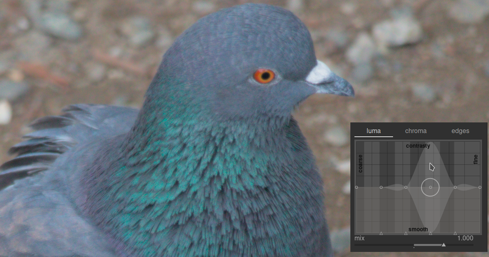
The following image shows the default state of the contrast equalizer module before any adjustments have been made:
Raising the two control points at the right-hand end of the graph will increase the sharpness of the fine details (the eye and feathers of the bird) while leaving coarser details (the rocks in the background) largely unaffected. The example below has been exaggerated to better illustrate the effect.
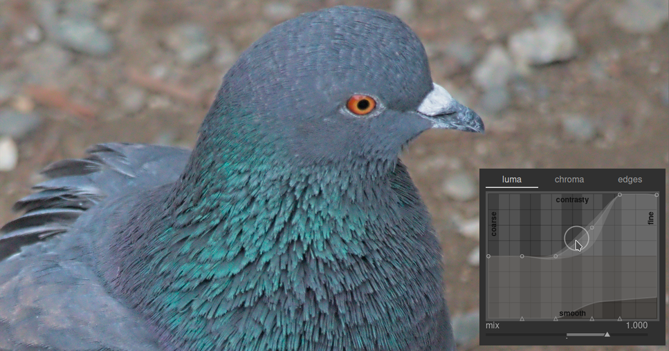
Increasing the local contrast can also amplify the luma noise in the image. A second spline located at the bottom of the graph can be used used to denoise the selected detail scales. Raise this spline (by clicking just above one of the triangles at the bottom of the graph and dragging the line upwards) to reduce noise at the given wavelet scale. In the example above, the dark denoising spline has been raised at the fine-detail end of the graph.
🔗chroma tab
The chroma tab allows the color contrast or saturation to be adjusted at the selected wavelet scales. See the following example:
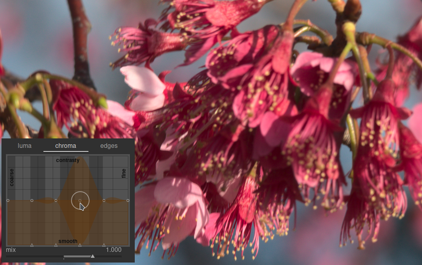
Say you wanted to bring out the green color of the anthers at the end of the stamen. The pink petals of the flowers are already quite saturated, but using contrast equalizer you can selectively boost the saturation on the small scale of the anthers without impacting the saturation of the petals. By raising the third control point from the right, you can target the saturation of the anthers only:

As in the luma tab, the chroma tab also has a denoising spline at the bottom of the graph. This can be used to handle chroma noise at different scales within the image. Chroma denoising can generally be more aggressive on larger wavelet scales and has less effect on a smaller scale.
🔗edge tab
The basic wavelet à trous transform has been enhanced in the contrast equalizer to be “edge-aware”, which can help to reduce the gradient reversals and halo artifacts that the basic algorithm can produce. The edges tab does not directly act on the edges in an image; rather it adjusts the edge awareness feature of the wavelet transform. If you have not adjusted the luma or chroma splines, adjusting the edge awareness spline will have no effect.
To see the sorts of artifacts that the edges curve tries to combat, here is an example taken from the original paper “Edge-Optimized À-Trous Wavelets for Local Contrast Enhancement with Robust Denoising” (Hanika, Damertz and Lensch 2011):
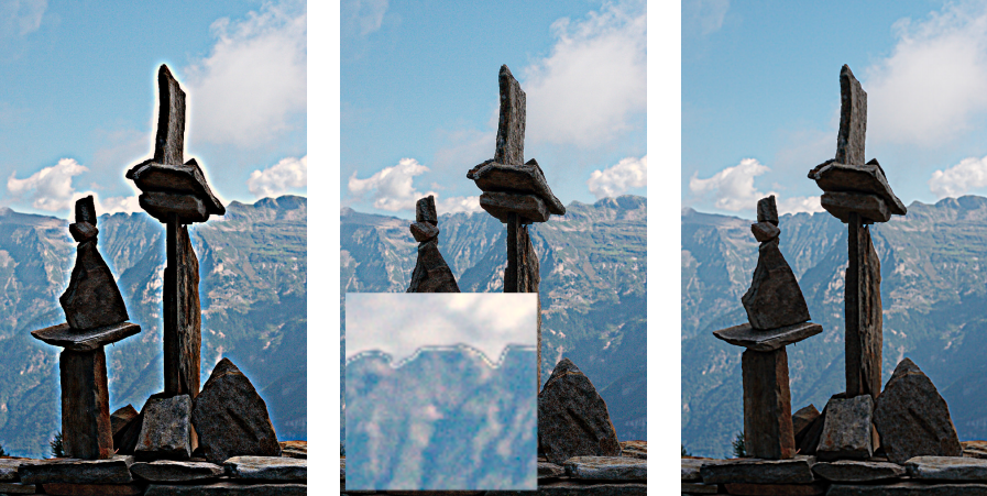
In the image on the left, the edges spline has been reduced to a minimum, effectively disabling the edge awareness and resulting in halos. In the middle image, the edges spline has been increased too much, resulting in gradient reversals. In the image on the right the edges spline has been set somewhere in between the two extremes, resulting in nice clean edges.
Usually the default central position of the spline is a good starting point, but if there are objectionable artifacts around the edges, this control can be helpful in mitigating them. Some experimentation will be required.