color calibration

A fully-featured color-space correction, white balance adjustment and channel mixer module.

This simple yet powerful module can be used in the following ways:

To adjust the white balance (chromatic adaptation), working in tandem with the white balance module. Here, the white balance module makes some initial adjustments (required for the demosaic module to work effectively), and the color calibration module then calculates a more perceptually-accurate white balance after the input color profile has been applied.
As a simple RGB channel mixer, adjusting the R, G and B output channels based on the R, G and B input channels, to perform cross-talk color-grading.
To adjust the color saturation and brightness of the image, based on the relative strength of the R, G and B channels of each pixel.
To produce a grayscale output based on the relative strengths of the R, G and B channels, in a way similar to the response of black and white film to a light spectrum.
To improve the color accuracy of the input color profile using a color checker chart.

🔗White Balance in the Chromatic Adaptation Transformation (CAT) tab

Chromatic adaptation aims to predict how all surfaces in the scene would look if they had been lit by another illuminant. What we actually want to predict, though, is how those surfaces would have looked if they had been lit by the same illuminant as your monitor, in order to make all colors in the scene match the change of illuminant. White balance, on the other hand, aims only at ensuring that whites and grays are really neutral (R = G = B) and doesn’t really care about the rest of the color range. White balance is therefore only a partial chromatic adaptation.

Chromatic adaptation is controlled within the Chromatic Adaptation Transformation (CAT) tab of the color calibration module. When used in this way the white balance module is still required as it needs to perform a basic white balance operation (connected to the input color profile values). This technical white balancing (“camera reference” mode) is a flat setting that makes grays lit by a standard D65 illuminant look achromatic, and makes the demosaicing process more accurate, but does not perform any perceptual adaptation according to the scene. The actual chromatic adaptation is then performed by the color calibration module, on top of those corrections performed by the white balance and input color profile modules. The use of custom matrices in the input color profile module is therefore discouraged. Additionally, the RGB coefficients in the white balance module need to be accurate in order for this module to work in a predictable way.

The color calibration and white balance modules can be automatically applied to perform chromatic adaptation for new edits by setting the chromatic adaptation workflow option (preferences > processing > auto-apply chromatic adaptation defaults) to “modern”. If you prefer to perform all white balancing within the white balance module, a “legacy” option is also provided. Neither option precludes the use of other modules (such as color balance RGB) for creative color grading further along the pixel pipeline.

By default, color calibration performs chromatic adaptation by:

reading the RAW file’s Exif data to fetch the scene white balance set by the camera,
adjusting this setting using the camera reference white balance from the white balance module,
further adjusting this setting with the input color profile in use (standard matrix only).

For consistency, the color calibration module’s default settings always assume that the standard matrix is used in the input color profile module – any non-standard settings in this module are ignored. However, color calibration’s defaults can read any auto-applied preset in the white balance module.

It is also worth noting that, unlike the white balance module, color calibration can be used with masks. This means that you can selectively correct different parts of the image to account for differing light sources.

To achieve this, create an instance of the color calibration module to perform global adjustments using a mask to exclude those parts of the image that you wish to handle differently. Then create a second instance of the module reusing the mask from the first instance (inverted) using a raster mask.

🔗CAT tab workflow

The default illuminant and color space used by the chromatic adaptation are initialised from the Exif metadata of the RAW file. There are four options available in the CAT tab to set these parameters manually:

Use the color-picker (to the right of the color patch) to select a neutral color from the image or, if one is unavailable, select the entire image. In this case, the algorithm finds the average color within the chosen area and sets that color as the illuminant. This method relies on the “gray-world” assumption, which predicts that the average color of a natural scene will be neutral. This method will not work for artificial scenes, for example those with painted surfaces.
Select “(AI) detect from edges”, which uses a machine-learning technique to detect the illuminant using the entire image. This algorithm finds the average gradient color over the edges in the image and sets that color as the illuminant. This method relies on the “gray-edge” assumption, which may fail if large chromatic aberrations are present. As with any edge-detection method, it is sensitive to noise and poorly suited to high-ISO images, but it is very well suited for artificial scenes where no neutral colors are available.
Select “(AI) detect from surfaces”, which combines the two previous methods, also using the entire image. This algorithm finds the average color within the image, giving greater weight to areas where sharp details are found and colors are strongly correlated. This makes it more immune to noise than the edge variant and more immune to legitimate non-neutral surfaces than the naïve average, but sharp colored textures (like green grass) are likely to make it fail.
Select “as shot in camera” to restore the camera defaults and re-read the RAW Exif.

The color patch shows the color of the currently calculated illuminant projected into sRGB space. The aim of the chromatic adaptation algorithm is to turn this color into pure white, which does not necessarily means shifting the image toward its perceptual opponent color. If the illuminant is properly set, the image will be given the same tint as shown in the color patch when the module is disabled.

To the left of the color patch is the CCT (correlated color temperature) approximation. This is the closest temperature, in kelvin, to the illuminant currently in use. In most image processing software it is customary to set the white balance using a combination of temperature and tint. However, when the illuminant is far from daylight, the CCT becomes inaccurate and irrelevant, and the CIE (International Commission on Illumination) discourages its use in such conditions. The CCT reading informs you of the closest CCT match found:

When the CCT is followed by “(daylight)”, this means that the current illuminant is close to an ideal daylight spectrum ± 0.5 %, and the CCT figure is therefore meaningful. In this case, you are advised to use the “D (daylight)” illuminant.
When the CCT is followed by “(black body)”, this means that the current illuminant is close to an ideal black body (Planckian) spectrum ± 0.5 %, and the CCT figure is therfore meaningful. In this case, you are advised to use the “Planckian (black body)” illuminant.
When the CCT is followed by “(invalid)”, this means that the CCT figure is meaningless and wrong, because we are too far from either a daylight or a black body light spectrum. In this case, you are advised to use the custom illuminant. The chromatic adaptation will still perform as expected (see the note below), so the “(invalid)” tag only means that the current illuminant color is not accurately tied to the displayed CCT. This tag is nothing to be concerned about – it is merely there to tell you to stay away from the daylight and planckian illuminants because they will not behave as you might expect.

When one of the above illuminant detection methods is used, the module checks where the calculated illuminant sits using the two idealized spectra (daylight and black body) and chooses the most accurate spectrum model to use in its illuminant parameter. The user-interface will change accordingly:

A temperature slider will be provided if the detected illuminant is close to a D (daylight) or Planckian (black body) spectrum, for which the CCT is meaningful.
Hue and chroma sliders in CIE 1976 Luv space are offered for the custom illuminant, which allows direct selection of the illuminant color in a perceptual framework without any intermediate assumption.

Note: Internally, the illuminant is represented by its absolute chromaticity coordinates in CIE xyY color space. The illuminant selection options in the module are merely interfaces to set up this chromaticity from real-world relationships and are intended to make this process faster. It does not matter to the algorithm if the CCT is tagged “invalid” – this just means that the relationship between the CCT and the corresponding xyY coordinates is not physically accurate. Regardless, the color set for the illuminant, as displayed in the patch, will always be honored by the algorithm.

When switching from one illuminant to another, the module attempts to translate the previous settings to the new illumninant as accurately as possible. Switching from any illuminant to custom preserves your settings entirely, since the custom illuminant is a general case. Switching between other modes, or from custom to any other mode, will not precisely preserve your settings from the previous mode due to rounding errors.

Other hard-coded illuminants are available (see below). Their values come from standard CIE illuminants and are absolute. You can use them directly if you know exactly what kind of light bulb was used to illuminate the scene and if you trust your camera’s input profile and reference (D65) coefficients to be accurate. Otherwise, see caveats below.

🔗CAT tab controls

adaptation

The working color space in which the module will perform its chromatic adaptation transform and channel mixing. The following options are provided:

Linear Bradford (1985): This is accurate for illuminants close to daylight and is compatible with the ICC v4 standard, but produces out-of-gamut colors for more difficult illuminants.

CAT16 (2016): This is the default option and is more robust in avoiding imaginary colors while working with large gamut or saturated cyan and purple. It is more accurate than the Bradford CAT in most cases.

Non-linear Bradford (1985): This can sometimes produce better results than the linear version but is unreliable.

XYZ: This is the least accurate method and is generally not recommended except for testing and debugging purposes.

none (disable): Disable any adaptation and use the pipeline working RGB space.

illuminant

The type of illuminant assumed to have lit the scene. Choose from the following:

same as pipeline (D50): Do not perform chromatic adaptation in this module instance but just perform channel mixing, using the selected adaptation color space.

CIE standard illuminant: Choose from one of the CIE standard illuminants (daylight, incandescent, fluorescent, equi-energy, or black body), or a non-standard “LED light” illuminant. These values are all pre-computed – as long as your camera sensor is properly profiled, you can just use them as-is. For illuminants that lie near the Planckian locus, an additional “temperature” control is also provided (see below).

custom: If a neutral gray patch is available in the image, the color of the illuminant can be selected using the color picker, or can be manually specified using hue and saturation sliders (in LCh perceptual color space). The color swatch next to the color picker shows the color of the calculated illuminant used in the CAT compensation. The color picker can also be used to restrict the area used for AI detection (below).

(AI) detect from image surfaces: This algorithm obtains the average color of image patches that have a high covariance between chroma channels in YUV space and a high intra-channel variance. In other words, it looks for parts of the image that appear as though they should be gray, and discards flat colored surfaces that may be legitimately non-gray. It also discards chroma noise as well as chromatic aberrations.

(AI) detect from image edges: Unlike the white balance module’s auto-white-balancing which relies on the “gray world” assumption, this method auto-detects a suitable illuminant using the “gray edge” assumption, by calculating the Minkowski p-norm (p = 8) of the laplacian and trying to minimize it. That is to say, it assumes that edges should have the same gradient over all channels (gray edges). It is more sensitive to noise than the previous surface-based detection method.

as shot in camera: Calculate the illuminant based on the white balance settings provided by the camera.

temperature

Adjust the color temperature of the illuminant. Move the slider to the right to assume a more blue illuminant, which will make the white-balanced image appear warmer/more red. Move the slider to the left to assume a more red illuminant, which makes the image appear cooler/more blue after compensation.

This control is only provided for illuminants that lie near the Planckian locus and provides fine-adjustment along that locus. For other illuminants the concept of “color temperature” doesn’t make sense, so no temperature slider is provided.

hue

For custom white balance, set the hue of the illuminant color in LCh color space (derived from CIE Luv space).

chroma

For custom white balance, set the chroma (or saturation) of the illuminant color in LCh color space (derived from CIE Luv space).

gamut compression

Most camera sensors are slightly sensitive to invisible UV wavelengths, which are recorded on the blue channel and produce “imaginary” colors. Once corrected by the input color profile, these colors will end up out of gamut (that is, it may no longer be possible to represent certain colors as a valid [R,G,B] triplet with positive values in the working color space) and produce visual artifacts in gradients. The chromatic adaptation may also push other valid colors out of gamut, at the same time pushing any already out-of-gamut colors even further out of gamut.

Gamut compression uses a perceptual, non-destructive, method to attempt to compress the chroma while preserving the luminance as-is and the hue as close as possible, in order to fit the whole image into the gamut of the pipeline working color space. One example where this feature is very useful is for scenes containing blue LED lights, which are often quite problematic and can result in ugly gamut clipping in the final image.

clip negative RGB from gamut

Remove any negative RGB values (set them to zero). This helps to deal with bad black level as well as the blue channel clipping issues that may occur with blue LED lights. This option is destructive for color (it may change the hue) but ensures a valid RGB output no matter what. It should never be disabled unless you want to take care of the gamut mapping manually and understand what you are doing. In that case, use the black level correction in the exposure module to get rid of any negative RGB (RGB means light, which is energy, and which should always be a positive quantity), then increase the gamut compression until no solid black patches remain in the image. Proper denoising may help getting rid of odd RGB values too. Note that this approach may still be insufficient to recover some deep and luminous shades of blue.

Note 1: It has been reported that some OpenCL drivers don’t play well when negative RGB are present in the pixel pipeline, because many pixel operators use logarithms and power functions (filmic, color balance, all the CIE Lab <-> CIE XYZ color space conversions), which are not defined for negative numbers. Although the inputs are sanitized before sensitive operations, it is not enough for some OpenCL drivers, which will output isolated NaN (Not a Number) values. These NaN values may be subsequently spread by local filters (blurring and sharpening operations, like sharpness, local contrast, contrast equalizer, low pass, high pass, surface blur, and filmic highlights reconstruction), resulting in large black, grey or white squares.

In all these cases, you must enable the “clip negative RGB from gamut” option in the color calibration module.

Note 2: A common case for failure of the color algorithms in color calibration (especially the gamut compression) is pixels that have a luminance value of 0 (Y channel of the CIE 1931 XYZ space), but non-zero chromaticity values (X and Z channels of the CIE 1931 XYZ space). This case is a numerical oddity that matches no physical reality (a pixel with no luminance should have no chromaticity either), will produce a division by zero in xyY and Yuv color spaces, and will create NaN RGB values as a result. This issue is not corrected inside color calibration because it is a symptom of a bad input profiling and/or a bad black point level, and needs to be addressed manually either by adjusting the input color profile with the channel mixer or in the exposure module’s black level correction.

🔗CAT warnings

The chromatic adaptation in this module relies on a number of assumptions about the earlier processing steps in the pipeline in order to work correctly, and it can be easy to inadvertently break those assumptions in subtle ways. To help you to avoid these kinds of mistakes, the color calibration module will show warnings in the following circumstances.

If the color calibration module is set up to perform chromatic adaptation but the white balance module is not set to “camera reference”, warnings will be shown in both modules. These errors can be resolved either by setting the white balance module to “camera reference” or by disabling chromatic adaptation in the color calibration module. Note that some sensors may require minor corrections within the white balance module in which case these warnings can be ignored.
If two or more instances of color calibration have been created, each attempting to perform chromatic adaptation, an error will be shown on the second instance. This could be a valid use case (for instance where masks have been set up to apply different white balances to different non-overlapping areas of the image) in which case the warnings can be ignored. For most other cases, chromatic adaptation should be disabled in one of the instances to avoid double-corrections.

By default, if an instance of the color calibration module is already performing chromatic adaptation, each new instance you create will automatically have its adaptation set to “none (bypass)” to avoid this “double-correction” error.

The chromatic adaptation modes in color calibration can be disabled by either setting the adaptation to “none (bypass)” or setting the illuminant to “same as pipeline (D50)” in the CAT tab.

These warnings are intended to prevent common and easy mistakes while using the automatic default presets in the module in a typical RAW editing workflow. When using custom presets and some specific workflows, such as editing film scans or JPEGs, these warnings can and should be ignored.

Advanced users can disable module warnings in preferences > processing > show warning messages.

🔗channel mixing

The remainder of this module is a standard channel mixer, allowing you to adjust the output R, G, B, colorfulness, brightness and gray of the module based on the relative strengths of the R, G and B input channels.

Channel mixing is performed in the color space defined by the adaptation control on the CAT tab. For all practical purposes, these CAT spaces are particular RGB spaces tied to human physiology and proportional to the light emissions in the scene, but they still behave in the same way as any other RGB space. The use of any of the CAT spaces can make the channel mixer tuning process easier, due to their connection with human physiology, but it is also possible to mix channels in the RGB working space of the pipeline by setting the adaptation to “none (bypass)”. To perform channel mixing in one of the adaptation color spaces without chromatic adaptation, set the illuminant to “same as pipeline (D50)”.

Note: The actual colors of the CAT or RGB primaries used for the channel mixing, projected to sRGB display space, are painted in the background of the RGB sliders, so you can get a sense of the color shift that will result from your altered settings.

Channel mixing is a process that defines a boosting/muting factor for each channel as a ratio of all the original channels. Instead of entering a single flat correction that ties the output value of a channel to its input value (for example, R_output = R_input × correction), the correction to each channel is dependent on the input of all of the channels for each pixel (for example, R_output = R_input × R_correction + G_input × G_correction + B_input × B_correction). Thus a pixel’s channels contribute to each other (a process known as “cross-talk”) which is equivalent to rotating the primary colors of the color space in 3D. This is, in effect, digital simulation of physical color filters.

Although rotating primary colors in 3D is ultimately equivalent to applying a general hue rotation, the connection between the RGB corrections and the resulting perceptual hue rotation is not directly predictable, which makes the process non-intuitive. “R”, “G” and “B” should be taken as a mixture of 3 lights that we dial up and down, not as a set of colors or hues. Also, since RGB tristimulus does not decouple luminance and chrominance, but is an additive lighting setup, the “G” channel is more strongly tied to human luminance perception than the “R” and “B” ones. All pixels have a non-zero G channel, which implies that any correction to the G channel is likely to affect all pixels.

The channel mixing process is therefore tied to a physical interpretation of the RGB tristimulus (as additive lights), which makes it well-suited for primary color grading and illuminant corrections, and blends the color changes smoothly. However, trying to understand and predict it from a perceptual point of view (luminance, hue and saturation) is going to fail and is discouraged.

Note: The “R”, “G” and “B” labels on the channels of the color spaces in this module are merely conventions formed out of habit. These channels do not necessarily look “red”, “green” and “blue”, and users are advised against trying to make sense out of them based on their names. This is a general principle that applies to any RGB space used in any application.

🔗R, G and B tabs

At its most basic level, you can think of the R, G and B tabs of the color calibration module as a type of matrix multiplication between a 3x3 matrix and the input [R G B] values. This is in fact very similar to what a matrix-based ICC color profile does, except that the user can input the matrix coefficients via the darktable GUI rather than reading the coefficients from an ICC profile file.

┌ R_out ┐     ┌ Rr Rg Rb ┐     ┌ R_in ┐
│ G_out │  =  │ Gr Gg Gb │  X  │ G_in │
└ B_out ┘     └ Br Bg Bb ┘     └ B_in ┘

If, for example, you’ve been provided with a matrix to transform from one color space to another, you can enter the matrix coefficients into the channel mixer as follows:

select the R tab and then set the Rr, Rg & Rb values using the R, G and B input sliders
select the G tab and then set the Gr, Gg & Gb values using the R, G and B input sliders
select the B tab and then set the Br, Bg & Bb values using the R, G and B input sliders

By default, the mixing function in color calibration just copies the input [R G B] channels straight over to the matching output channels. This is equivalent to multiplying by the identity matrix:

┌ R_out ┐     ┌ 1  0  0 ┐      ┌ R_in ┐
│ G_out │  =  │ 0  1  0 │   X  │ G_in │
└ B_out ┘     └ 0  0  1 ┘      └ B_in ┘

For a more intuitive understanding of how the mixing sliders on the R, G and B tabs behave, consider the following:

for the R destination channel, adjusting sliders to the right will make the R, G or B areas of the image more “red”. Moving the slider to the left will make those areas more “cyan”.
for the G destination channel, adjusting sliders to the right will make the R, G or B areas of the image more “green”. Moving the slider to the left will make those areas more “magenta”.
for the B destination channel, adjusting sliders to the right will make the R, G or B areas of the image more “blue”. Moving the slider to the left will make those areas more “yellow”.

🔗R, G and B tab controls

The following controls are shown for each of the R, G and B tabs:

input R/G/B: Choose how much the input R, G and B channels influence the output channel relating to the tab concerned.
normalize channels: Select this checkbox to normalize the coefficients to try to preserve the overall brightness of this channel in the final image as compared to the input image.

🔗brightness and colorfulness tabs

The brightness and colorfulness (color saturation) of pixels in an image can also be adjusted based on the R, G and B input channels. This uses the same basic algorithm that the filmic rgb module uses for tone mapping (which preserves RGB ratios) and for mid-tones saturation (which massages them).

saturation algorithm: This control allows you to upgrade the saturation algorithm to the new 2021 version, for edits produced prior to darktable 3.6 – it will not appear for edits that already use the latest version.

🔗colorfulness tab controls

input R/G/B: Adjust the color saturation of pixels, based on the R, G and B channels of those pixels. For example, adjusting the input R slider will affect the color saturation of pixels containing a lot of “R” more than pixels containing only a small amount of “R”.
normalize channels: Select this checkbox to try to keep the overall saturation constant between the input and output images.

🔗brightness tab controls

input R/G/B: Adjust the brightness of certain colors in the image, based on the R, G and B channels of those colors. For example, adjusting the input R slider will affect the brightness of colors containing a lot of R channel much more than colors containing only a small amount of R channel. When darkening/brightening a pixel, the ratio of the R, G and B channels for that pixel is maintained, in order to preserve the hue.
normalize channels: Select this checkbox to try to keep the overall brightness constant between the input and output images.

🔗gray tab

Another very useful application of color calibration is the ability to mix the channels together to produce a grayscale output – a monochrome image. Select the gray tab, and set the R, G and B sliders to control how much each channel contributes to the brightness of the output. This is equivalent to the following matrix multiplication:

GRAY_out  =   [ r  g  b ]  X  ┌ R_in ┐
                              │ G_in │
                              └ B_in ┘

When dealing with skin tones, the relative weights of the three channels will affect the level of detail in the image. Placing more weight on R (e.g. [0.9, 0.3, -0.3]) will make for smooth skin tones, whereas emphasising G (e.g. [0.4, 0.75, -0.15]) will bring out more detail. In both cases the B channel is reduced to avoid emphasising unwanted skin texture.

🔗gray tab controls

input R/G/B: Choose how much each of the R, G and B channels contribute to the gray level of the output. The image will only be converted to monochrome if the three sliders add up to some non-zero value. Adding more B will tend to bring out more details, adding more R will tend to smooth skin tones.
normalize channels: Select this checkbox to try to keep the overall brightness constant as the sliders are adjusted.

🔗extracting settings using a color checker

Since the channel mixer is essentially an RGB matrix (similar to the input color profile used for RAW images) it can be used to improve the color accuracy of the input color profile by computing ad-hoc color calibration settings.

These computed settings aim to minimize the color difference between the scene reference and the camera recording in a given lighting situation. This is equivalent to creating a generic ICC color profile but here, the profile is instead stored as module settings that can be saved as presets or styles, to be shared and re-used between images. Such profiles are meant to complement and refine the generic input profile but do not replace it.

This feature can assist with:

handling difficult illuminants, such as low CRI light bulbs, for which a mere white balancing will never suffice,
digitizing artworks or commercial products where an accurate rendition of the original colors is required,
neutralizing a number of different cameras to the same ground-truth, in multi-camera photo sessions, in order to obtain a consistent base look and share the color editing settings with a consistent final look,
obtaining a sane color pipeline from the start, nailing white balance and removing any bounced-light color cast at once, with minimal effort and time.

🔗supported color checker targets

Users are not currently permitted to use custom targets, but a limited number of verified color checkers (from reputable manufacturers) are supported:

X-Rite / Gretag MacBeth Color Checker 24 (pre- and post-2014),
Datacolor SpyderCheckr 24,
Datacolor SpyderCheckr 48.

Users are discouraged from obtaining cheap, off-brand, color targets as color constancy between batches cannot possibly be asserted at such prices. Inaccurate color checkers will only defeat the purpose of color calibration and possibly make things worse.

IT7 and IT8 charts are not supported since they are hardly portable and not practical for use on-location for ad-hoc profiles. These charts are better suited for creating generic color profiles, undertaken using a standard illuminant, for example with Argyll CMS.

Note: X-Rite changed the formula of their pigments in 2014, which slightly altered the color of the patches. Both formulas are supported in darktable, but you should be careful to choose the correct reference for your target. If in doubt, try both and choose the one that yields the lowest average delta E after calibration.

🔗prerequisites

In order to use this feature you will need to take a test shot of a supported color checker chart, on-location, under appropriate lighting conditions:

frame the chart in the center 50% of the camera’s field, to ensure that the image is free of vignetting,
ensure that the main light source is far enough from the chart to give an even lighting field over the surface of the chart,
adjust the angle between the light, chart and lens to prevent reflections and gloss on the color patches,
for the best quality profile you should capture an image with the appropriate brightness. To achieve this, take a few bracketed images (between -1 and +1 EV) of your color checker and load them into darktable, ensuring that all modules between color calibration and output color profile are disabled. Choose the image where the white patch has a brightness L of 94-96% in CIE Lab space or a luminance Y of 83-88% in CIE XYZ space (use the global color picker). This step is not strictly necessary – alternatively you can take a single image and apply the exposure compensation as recommended in the profile report.

If the lighting conditions are close to a standard D50 to D65 illuminant (direct natural light, no colored bounced light), the color checker shot can be used to produce a generic profile that will be suitable for any daylight illuminant with only a slight adjustment of the white balance.

If the lighting conditions are peculiar and far from standard illuminants, the color checker shot will be only usable as an ad-hoc profile for pictures taken in the same lighting conditions.

🔗usage

The settings used in color calibration depend on the chosen CAT space and on any color settings defined earlier in the pipe within the white balance and input color profile modules. As such, the results of the profiling (e.g. the RGB channel mixing coefficients) are valid only for a rigid set of CAT space, white balance and input color profile settings. If you wish to create a generic style with your profile, don’t forget that you will need to include the settings from these modules as well.

Use the following process to create your profile preset/style:

Enable the lens correction module to correct any vignetting that might mislead the calibration,
On the bottom of the color calibration module, click on the arrow near the calibrate with a color checker label, to show the controls,
Pick the correct model and manufacturer of your color checker from the chart drop-down,
In the image preview, an overlay of the chart’s patches will appear. Drag the corners of the chart so that they match the visual references (dots or crosses) around the target, to compensate for any perspective distortion,
Click the refresh button to compute the profile,
Check the Profile quality report. If it is “good”, you can click on the validation button. If not, try changing the optimization strategy and refresh the profile again.
Save the profile in a preset or style, or simply copy & paste the module settings to all of the pictures taken under the same lighting conditions, from within the lighttable view or filmstrip.

Note: You don’t need to use the standard matrix in the input color profile module when performing a calibration, but be aware that the “as shot in camera” default white balance will not work properly with any other profile, and that you will need to always use the same input profile whenever you reuse such calibration settings.

🔗reading the profile report

The profile report helps you to assess the quality of the calibration. The settings in color calibration are only a “best fit” optimization and will never be 100% accurate for the whole color spectrum. We therefore need to track “how inaccurate” it is in order to know whether we can trust this profile or not.

Bad profiles can happen and will do more harm than good if used.

🔗delta E and the quality report

The CIE delta E 2000 (ΔE) is used as a perceptual metric of the error between the reference color of the patches and the color obtained after each step of calibration:

ΔE = 0 means that there is no error – the obtained color is exactly the reference color. Unfortunately, this will never happen in practice.
ΔE = 2.3 is defined as the Just Noticeable Difference (JND).
ΔE < 2.3 means that the average observer will not be able to tell the difference between the expected reference color and the obtained color. This is a satisfactory result.
ΔE > 2.3 means that the color difference between the expected reference and the obtained color is noticeable for the average observer. This is unsatisfactory but sometimes unavoidable.

The quality report tracks the average and maximum ΔE at the input of the module (before anything is done), after the chromatic adaptation step (white balance only), and at the output of the module (white balance and channel mixing). At each step, the ΔE should be lower than at the previous step, if everything goes as planned.

🔗profile data

The data generated by the profiling process comprises the RGB 3×3 matrix and the detected illuminant. These are expressed in the CAT adaptation space defined in the CAT tab and are provided in case you want to export these coefficients to other software. If the detected illuminant is daylight or black body, the matrix should be fairly generic and re-usable for other daylight and black body illuminants with the addition of a small white balance adjustment.

🔗normalization values

These are the settings that you should define, as-is, for the exposure and black level correction parameters in the exposure module, in order to obtain the lowest possible error in your profile. This step is optional and is useful only when the utmost precision is required, but beware that it can produce negative RGB values that will be clipped at various points in the pipeline.

🔗overlay

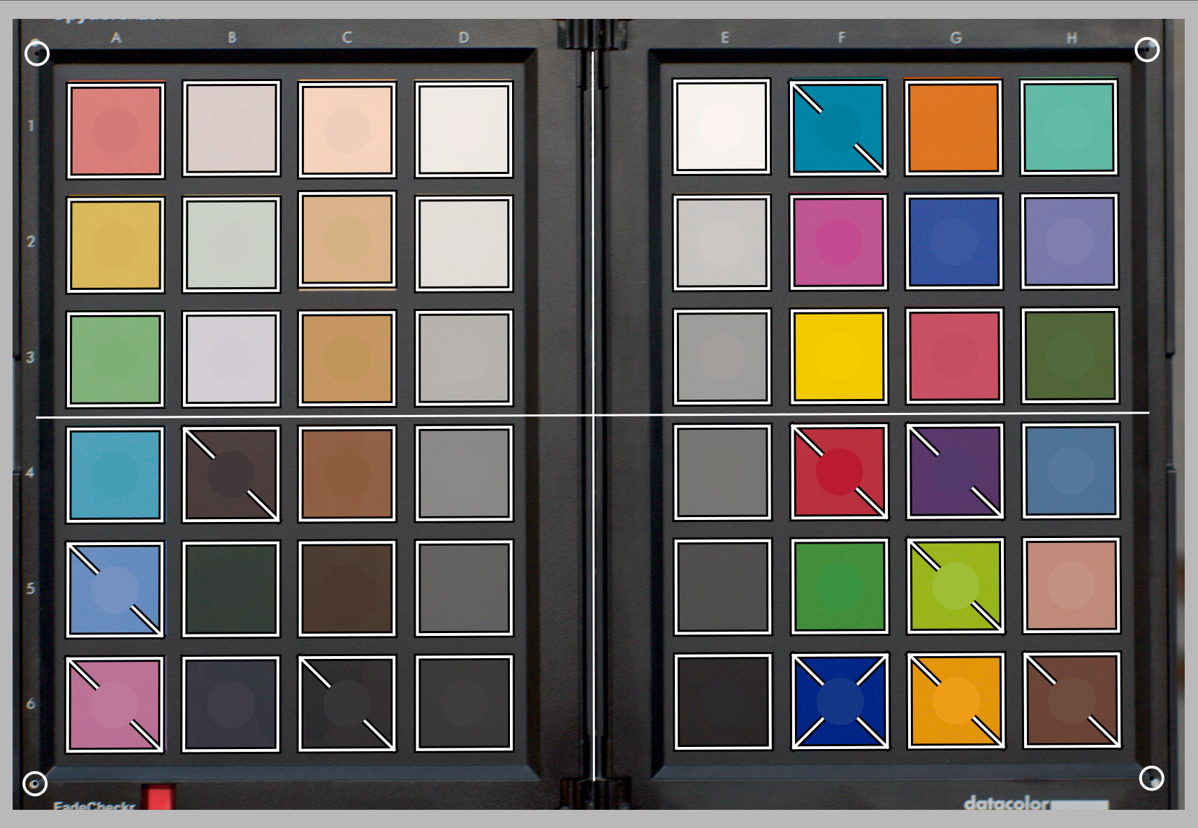
The chart overlay displays a disc in the center of each color patch, which represents the expected reference value of that patch, projected into the display RGB space. This helps you to visually assess the difference between the reference and the actual color without having to bother with ΔE values. This visual clue will be reliable only if you set the exposure module as instructed in the normalization values of the profile report.

Once the profile has been calibrated, some of the square patches will be crossed in the background by one or two diagonals:

patches that are not crossed have ΔE < 2.3 (JND), meaning they are accurate enough that the average observer will be unable to notice the deviation,
patches crossed with one diagonal have 2.3 < ΔE < 4.6, meaning that they are mildly inaccurate,
patches crossed with two diagonals have ΔE > 4.6 (2 × JND), meaning that they are highly inaccurate.

This visual feedback will help you to set up the optimization trade-off to check which colors are more or less accurate.

🔗enhancing the profile

Because any calibration is merely a “best fit” optimization (using a weighted least-squares method) it is impossible to have all patches within our ΔE < 2.3 tolerance. Some compromise will therefore be required.

The optimize for parameter allows you to define an optimization strategy that attempts to increase the profile accuracy in some colors at the expense of others. The following options are available:

none: Don’t use an explicit strategy but rely on the implicit stategy defined by the color checker manufacturer. For example, if the color checker has mostly low-saturation patches, the profile will be more accurate for less-saturated colors.
neutral colors: Give priority to grays and less-saturated colors. This is useful for desperate cases involving cheap fluorescent and LED lightings, having low CRI. However, it may increase the error in highly-saturated colors more than not having any profile.
saturated colors: Give priority to primary colors and highly-saturated colors. This is useful in product and commercial photography, to get brand colors right.
skin and soil colors, foliage colors, sky and water colors: Give priority to the chosen hue range. This is useful if the subject of your pictures is clearly defined and has a typical color.
average delta E: Attempt to make the color error uniform across the color range and minimize the average perceptual error. This is useful for generic profiles.
maximum delta E: Attempt to minimize outliers and large errors, at the expense of the average error. This can be useful to get highly saturated blues back into line.

No matter what you do, strategies that favor a low average ΔE will usually have a higher maximum ΔE, and vice versa. Also, blues are always the more challenging color range to get correct, so the calibration usually falls back to protecting blues at the expense of everything else, or everything else at the expense of blues.

The ease of obtaining a proper calibration depends on the quality of the scene illuminant (daylight and high CRI illuminants should always be preferred), the quality of the primary input color profile, the black point compensation set in the exposure module, but first and foremost on the mathematical properties of the camera sensor’s filter array.

🔗profile checking

It is possible to use the color space check button (first on the left, at the bottom of the module) to perform a single ΔE computation of the color checker reference against the output of the color calibration module. This can be used in the following ways:

To check the accuracy of a profile calculated in particular conditions against a color checker shot in different conditions.
To evaluate the performance of any color correction performed earlier in the pipe, by setting the color calibration parameters to values that effectively disable it (CAT adaptation to none, everything else set to default), and just use the average ΔE as a performance metric.

🔗caveats

The ability to use standard CIE illuminants and CCT-based interfaces to define the illuminant color depends on sound default values for the standard matrix in the input color profile module as well as reasonable RGB coefficients in the white balance module.

Some cameras, most notably those from Olympus and Sony, have unexpected white balance coefficients that will always make the detected CCT invalid even for legitimate daylight scene illuminants. This error most likely comes from issues with the standard input matrix, which is taken from the Adobe DNG Converter.

It is possible to alleviate this issue, if you have a computer screen calibrated for a D65 illuminant, using the following process:

Display a white surface on your screen, for example by opening a blank canvas in any photo editing software you like
Take a blurry (out of focus) picture of that surface with your camera, ensuring that you don’t have any “parasite” light in the frame, you have no clipping, and are using an aperture between f/5.6 and f/8,
Open the picture in darktable and extract the white balance by using the spot tool in the white balance module on the center area of the image (non-central regions might be subject to chromatic aberrations). This will generate a set of 3 RGB coefficients.
Save a preset for the white balance module with these coefficients and auto-apply it to any color RAW image created by the same camera.